This article covers one of the most basic concepts in machine learning which is linear regression.

Table of Contents:

1. What is linear regression ?
2. The hypothesis function.
3. The cost function.
4. Gradient Descent.
5. Conclusion.

1- what is linear regression ?

Linear regression is a way to try and find a linear relationship between two variables, the idea may sound intimidating but all that it means is given some input variable like the weight of a person, linear regression can quantify the relative impact on this person’s height.

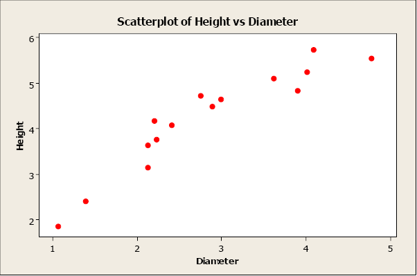
Of course, there’s no need to mention that before thinking about using linear regression we need to make sure that our data are linearly related , one way to do so is by plotting them on a graph and being able to visualize that the data follows approximately the shape of a straight line, like the figure below.

2- The hypothesis function:

As one of the first equation we learned in middle school, the linear equation is used to represent a straight line and looks like this:

Y = mx + b

where m is the slope and b is the intercept.

Now, the hypothesis function is  nothing but a linear equation with different notation:

where x is our input variable (weight) and the result is our output variable (height).

So, linear regression tries to find the best line that fits the data points, in other words it tries to find the parameters theta 0 and theta 1 where the cost function is at the lowest .

3- The cost function:

Having a set of data points that are linearly shaped, different lines could fit into them, and the criterion used to choose between the lines is the one whose cost function is the lowest.

the idea is quite intuitive, all that the function does is for each data point it calculates the squared difference between the predicted value calculated by our hypothesis function and the real corresponding value, these differences can be thought of as the distance between each point and its corresponding predicted on the graph as shown in the figure below.

it actually calculates the mean of these squared differences to ensure that it doesn’t depend on the number of elements in the training set.

So the question is, how do we choose theta0 and theta1 so that the cost function is minimized?

4- Gradient Descent:

Gradient Descent is an optimization algorithm used to minimize functions, in linear regression it is used to find the parameters theta0 and theta1 of our model to minimize our cost function J(Θ).

To simplify the concept a little bit, let’s suppose that our hypothesis function for a given problem depends only on one parameter theta1, meaning that theta0 is equal to 0.

we could for example calculate J(Θ) for a limited set of theta1 values, the plot below shows the behavior of the cost function in terms of theta1.

we can see that there is a global minimum of J(Θ1) when Θ1=1.

but that’s only using the naked eye, we need a way to find theta1 efficiently and this is where gradient descent comes to play.

The way gradient descent works is quite interesting , it starts with randomly initializing the parameter (s) theta1, calculates J(theta1) and keeps changing the parameter to reduce the cost function until we end up at a minimum.

The question is: how does it change the parameters ?

Well, it does so by applying the following algorithm:

where α is the learning rate, that is the size if the step in the direction of gradient and the derivative is the slope of the tangent line at the point theta1.

note: j=1, theta=theta1.

To get to the global minimum, we need to move in the direction of the slope, if it is negative we will ascend meaning theta which is represented by w in the above figure will increase , and if it is positive theta will decrease.

Now, we need to keep in mind that choosing the learning rate alpha is very critical because it shouldn’t be very large as the algorithm may overshoot the minimum and fail to converge, and shouldn’t be too small as it will take too much time to converge.

But all in all, if the cost function decreases in every iteration then the chosen alpha is perfect.

Now that we are familiar enough with gradient descent, let’s plug in the second parameter theta0, and remind ourselves with the formulas:

and after applying some calculus in calculating the derivatives we get :

where m is the size of the training set.

the plot of the cost function against theta0 and theta1 would look like this and it is called the surface plot.

here we can see that there’s a local optimum and a global optimum. the algorithm can converge to the local optimum and miss the global.

But, if we’re lucky our cost function could be a convex function and take the shape of a bowl, meaning there’s only one optimum.

Another way to plot the cost function is by the contour plot which looks like this:

here the points belonging to the same ‘circle’ or contour have the same value of cost, and the optimum is located right in the center.

5- Conclusion:

This was a humble article on linear regression with one variable, in the next part we will try to implement it using python.